在之前学习的时候,也有记录过如何数字信号处理的一些基础的知识,专栏的链接如下:
数字信号处理专栏。
感觉数字信号处理这些东西,每过一段时间最好还是回去好好温习一下,有些东西很长时间不用很容易就忘掉了。
今天主要是记录一下FFT的使用方法,在实际的使用的时候,虽然不一定需要自己去实现一个FFT的算法,在FPGA内部使用提供好的IP核就能够完成这些操作了。但是一些最基础的知识最好还是需要自己来掌握的。
1. 实信号和复信号的频谱的区别
简单来说,通过欧拉公式能够建立起实数和复数信号之间的联系。
对于实数信号,其在频域上的表现形式是在包含正负频率分量,以一个正弦信号为例,在正的频率处和负频率处都有频率分量。而对于复数信号,频率分量可以是只包含正的频率分量和负的频率分量。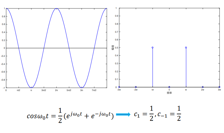
可以使用一段matlab代码来帮助理解。1
2
3
4
5
6
7
8
9
10
11
12
13
14
15
16
17
18
19
20
21
22
23
24
25
26
27
28
29
30
31
32
33
34
35
36
37
38
39
40
41
42
43
44
45
46
47
48
49
50
51
52
53% parameter define
fc = 1e6; % tone frequency
fs = 16e6; % sample rate
N = 8192; % samples in total
df = fs/N; % frequency resolution
n = 0:(N-1);
i_data = cos(2*pi*fc*n/fs);
q_data = sin(2*pi*fc*n/fs);
% generate a real signal
iq_real = complex(i_data, 0);
% using fft to analyse siganl
fft_real_signal = fft(iq_real);
abs_fft_real_signal = abs(fft(iq_real));
figure(1);
plot(real(fft_real_signal), imag(fft_real_signal));
title('复数坐标系显示实信号FFT输出共轭对称性');
ylabel('虚轴');
xlabel('实轴');
% change the x lable into MHz, for both side
% the real signal have both negative and postive frequency
x_index = 0:N-1;
x_index(x_index >= N/2) = x_index(x_index >= N/2) - N;
x_index = x_index.*df/1e6;
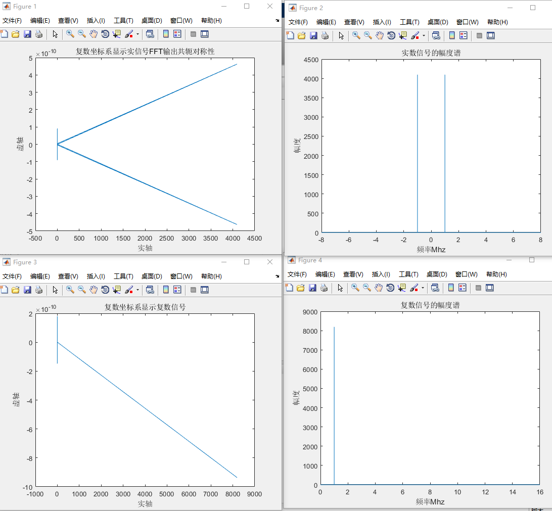
figure(2);
plot(x_index, abs_fft_real_signal);
title('实数信号的幅度谱');
ylabel('幅度');
xlabel('频率Mhz');
% generate a complex signal
iq_complex = complex(i_data, q_data);
% using fft to analyse siganl
fft_complex_signal = fft(iq_complex);
abs_fft_complex_signal = abs(fft(iq_complex));
figure(3);
plot(real(fft_complex_signal), imag(fft_complex_signal));
title('复数坐标系显示复数信号');
ylabel('虚轴');
xlabel('实轴');
% change the x lable into MHz, for both side
% the real signal have both negative and postive frequency
x_index = 0:N-1;
x_index = x_index.*df/1e6;
figure(4);
plot(x_index, abs_fft_complex_signal);
title('复数信号的幅度谱');
ylabel('幅度');
xlabel('频率Mhz');